Tutorial
- To investigate your genetic association study design, use the sliders and text boxes in the inputs section to select your parameters.
- Given your inputs, the calculated statistical power, expected disease allele frequencies, and probability of disease will be displayed in the results section.
- Change the independent variable at the top of the graphs section to visualize the change in power over the range of the selected parameter. All the other parameters remain as indicated in the inputs section. For the 'Cases + Controls' option indicating the total sample size, the ratio of cases to controls is specified by the calculation of 'Cases/Controls' in the inputs section.
- Click the menu at the top right hand side of graph to download plot and data.
- See below for parameter definitions and an example of how to use GAS Power Calculator.
- Click here to view the relevant equations used in calculating the results of GAS Power Calculator.
Definitions - Inputs
Cases:
Number of cases available to genotype for the study. Ranges from 100 to 100,000.
Controls:
Number of controls available to genotype for the study. Ranges from 100 to 100,000.
Signficance Level (\(\alpha\)):
Desired false positive rate per genetic marker. If all M markers are independent,
and you want a genome-wide false positive rate of x, the significance level should be \(\frac{x}{M}\) . Ranges from 1e-10 to 1.
Prevalence (prev):
Disease prevalence in the general population.
This is the probability that a randomly sampled individual has the disease. Ranges from 0.0001 to 1.
Disease Allele Frequency (DAF):
Frequency of the disease risk allele in the general population.
Disease allele frequency is usually higher in cases and lower in controls. Ranges from 0.0001 to 1.
Genotype Relative Risk (GRR):
The genotype relative risk depends on the disease model, where \(f_0, f_1,\) and \(f_2\) are the disease probabilities for
individuals with 0,1, or 2 copies of the disease risk allele. Ranges from 0.0001 to 1.
Multiplicative: \(GRR = \frac{f_1}{f_0} = \frac{f_2}{f_1}\)
Additive: \(GRR = \frac{f_1}{f_0}\)
Dominant: \(GRR = \frac{f_1}{f_0} = \frac{f_2}{f_0}\)
Recessive: \(GRR = \frac{f_2}{f_0} = \frac{f_2}{f_1}\)
Multiplicative: \(GRR = \frac{f_1}{f_0} = \frac{f_2}{f_1}\)
Additive: \(GRR = \frac{f_1}{f_0}\)
Dominant: \(GRR = \frac{f_1}{f_0} = \frac{f_2}{f_0}\)
Recessive: \(GRR = \frac{f_2}{f_0} = \frac{f_2}{f_1}\)
*Note: The lower bound for prevalence, disease allele frequency, and genotype relative risk is greater than 0 due to the fact that the study is irrelevant when there is no disease.
Definitions - Results
Expected power for a one-stage study (P):
Estimated statistical power given the input parameters. One-stage study (all samples genotyped on all markers in a single stage)
indicated since the CaTS power calculator version has two-stage study capability.
Expected disease allele frequency for cases (casesDAF):
Estimated frequency of the disease risk allele in the cases population.
Expected disease allele frequency for controls (controlsDAF):
Estimated frequency of the disease risk allele in the controls population.
Probability of disease for genotype A/A (with frequency AAfreq) (AAprob):
Probability that an individual with 2 copies of the disease risk allele will have the disease,
and the frequency of this genotype in the general population.
Probability of disease for genotype A/B (with frequency ABfreq) (ABprob):
Probability that an individual with 1 copy of the disease risk allele will have the disease,
and the frequency of this genotype in the general population.
Probability of disease for genotype B/B (with frequency BBfreq) (BBfreq):
Probability that an individual with 0 copies of the disease risk allele will have the disease,
and the frequency of this genotype in the general population.
Examples
The following is an example of how you could use the GAS Power Calculator.
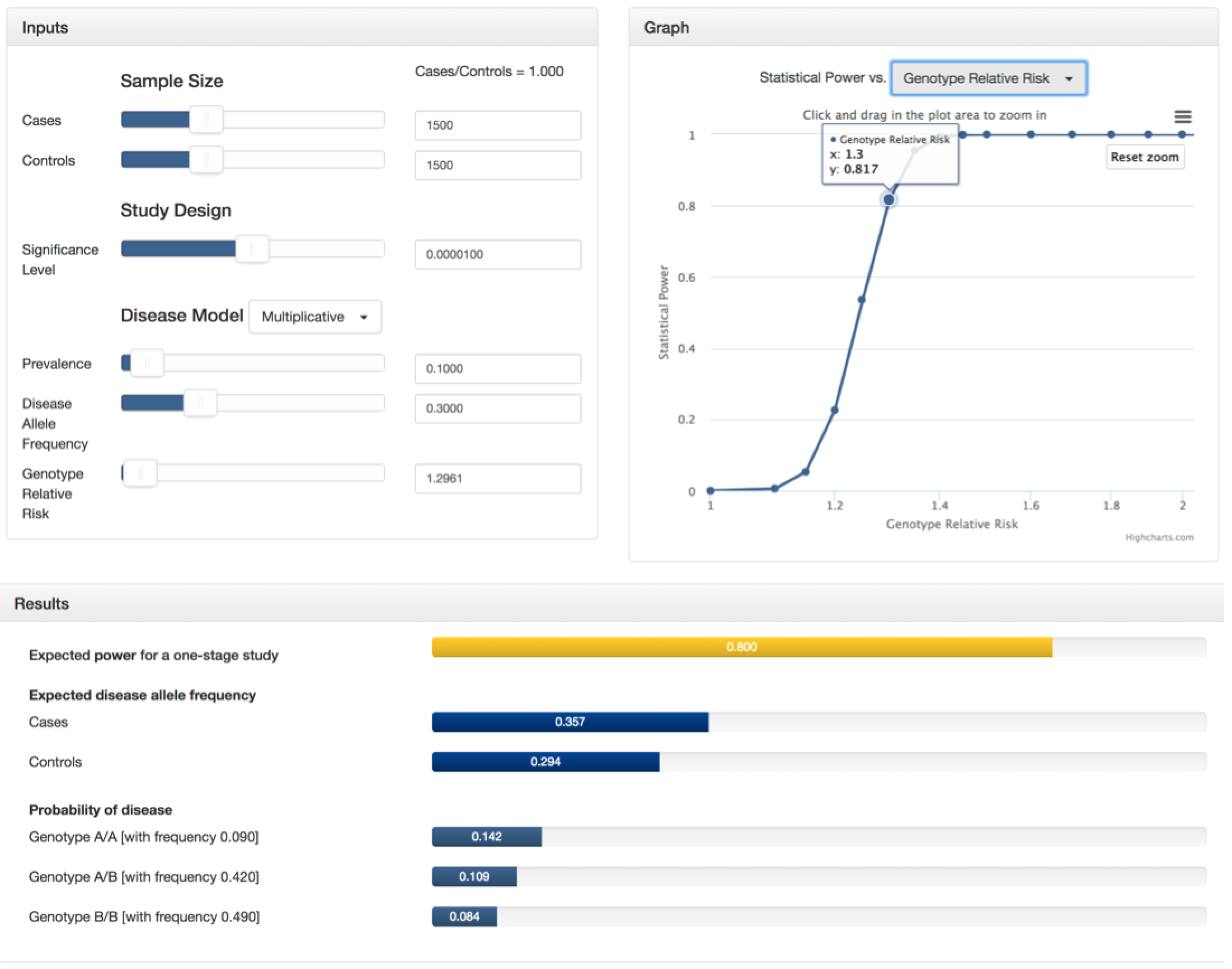
Suppose you are conducting a genome-wide association study with 1500 cases and 1500 controls. You plan to genotype these samples on 300,000 independent SNPs and are willing to tolerate a genome-wide false positive rate of 3. Therefore, your significance level will be 3/300000, or 0.00001. From previous studies, you know that the disease follows a multiplicative model and its prevalence is 0.10 with an allele frequency of 0.30 in the general population. Finally, you want determine the genotype relative risk that will result in a power of 0.80. To do this, you can select "Genotype Relative Risk" in the drop-down menu of the graph section and zoom in to see that a 0.80 power lies between a GRR of 1.295 and 1.3. At this point, use the GRR slider in the inputs section to estimate a more precise value (around GRR=1.2961). See the screenshots below or try it yourself!
Of course this is not the only application. Play around with the input values and the independent variable in the graph section to see how they influence the power of the study and the additional output values in the results section.