| |
PEDSTATS Tutorial -- Graphical Summary of Hardy-Weinberg Tests
When the --hardyWeinberg option is specified along with --pdf option, PEDSTATS will test each marker
in your data file for significant deviations from Hardy-Weinberg Equilibrium and summarize the results
graphically. If you aren't familiar with the test statistics used by PEDSTATS, you may find it helpful to
go over the section on Hardy-Weinberg Equilibrium testing first.
Graphical output for Chi-squared tests
The figure below shows the results of Hardy-Weinberg testing for a typical microsatellite marker (MARKER_1).
The numbers listed just below the title are the chi-squared test statistic
and associated p-value. For the MARKER_1 locus,
chi-squared is 28.59. The associated p-value for 15 degrees of freedom is 0.0182, indicating that allele frequencies for
MARKER_1 deviate significantly from Hardy-Weinberg equilibrium in this sample.
Since a significant HWE test result such as this may indicate genotyping error, a natural
follow-up would be to determine which genotype frequencies deviate significantly from their expected values.
To facilitate this process, we've included three additional panels that summarize the
expected, observed and residual values for each marker genotype cell used in the goodness-of-fit test.

The first panel on the left ("Observed") summarizes the genotype
distribution in the sample used to test MARKER_1 for Hardy-Weinberg equilibrium.
Values along the axes are allele ids. Possible values for the first allele in a genotype are listed along the
x-axis and those for the second allele can be found along the y-axis. PEDSTATS will occasionally pool alleles in order
to avoid small expected
counts. For the test of MARKER_1, there were six allele categories used; five of
these represent non-pooled alleles (5, 6, 7, 8 and 9). The sixth category represents a pool of
low-frequency alleles (2, 3, 4, 10 and 11) and is marked with a "P". The values in each cell are the observed counts for the associated
genotype; genotypes with high expected counts
are shaded dark blue while those lower expected counts are represented by lighter shades. You should
be able to verify that there were were 31 individuals homozygous for allele 5,
103 heterozygotes with genotype (6, 9) and total of 846 homozygotes in the sample.
The panel in the center ("Expected") shows the genotype distribution that would be expected in
the sample assuming Hardy-Weinberg equilibrium.
The counts in each cell are the expected cell values used for the chi-squared goodness of fit test. As before, cells that are shaded
dark blue have high expected counts and those with light blue shading have low expected counts. For the chi-squared test of MARKER_1,
the expected number of (5,5) homozygotes was 30.2, which is fairly close to the observed count of 31. On the other hand, the observed
count of 20 (5, 9) heterozygotes was quite different from the expected number of 41.2 individuals with this genotype.
The panel on the right ("Residuals") summarizes residual values. The number
in each cell
is the difference between the observed count and the expected count for each corresponding genotype. Each cell is shaded according to
the residual value defined as
Residualij = (Observedij - Expectedij) / sqrt(Expectedij)
When cell counts are sufficiently large, residuals will be approximately normally distributed with mean 0.0 and variance 1.0. Cells
shaded in red/orange tones have residual values that are more significant and therefore represent genotypes where the observed data
deviated significantly from Hardy-Weinberg equilibrium. Cells in lighter tones represent residual values that are relatively close to
their expected value of 0.0. For MARKER_1, counts for genotype (5, 9) appear to deviate significantly from what would be expected under
HWE; the cell corresponding to this genotype is shaded in red. Counts for (5,5) homozygotes only deviated slightly from expectations;
this is indicated by the light yellow shading for the corresponding residual cell.
Graphical output for exact tests
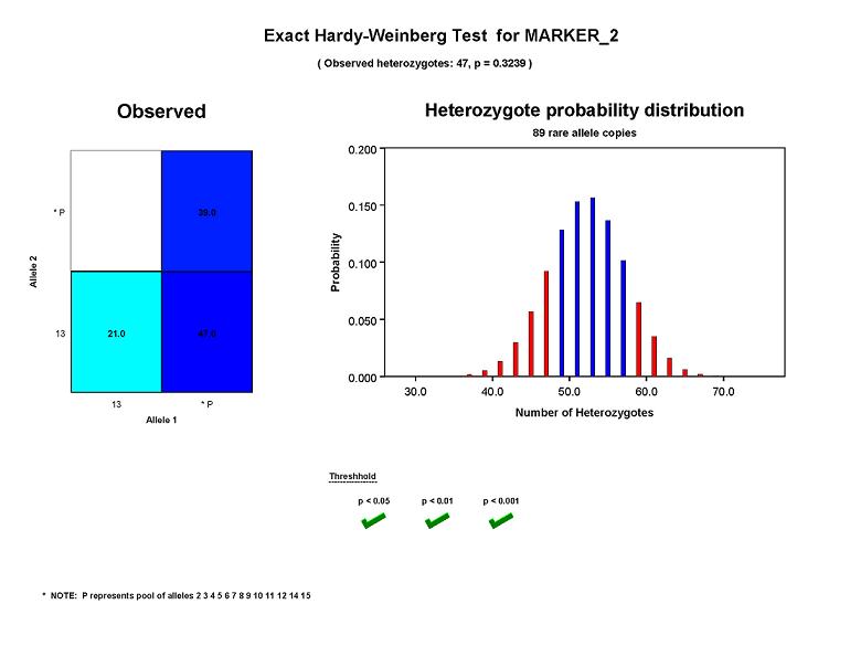
When an exact Hardy-Weinberg test is run, PEDSTATS will generate graphical output similar to the figure below .
In this case, a histogram is drawn to show the heterozygote probability distribution,
conditional on the number of rare allele copies (R) and the number of genotypes used for the test (N).
Bars shaded in red fall in the area of the distribution used to calculate the p-value.
The figure below shows results for an exact test of HWE using Marker_2, a microsatellite with 14 alleles ranging from 2
to 15. In order to avoid small cell counts that can be troublesome for an asymptotic test,
Pedstats has grouped all alleles except 13 into a single cell. Because there are two allele groups after pooling,
an exact test is run. After grouping, there are 89 copies of alleles belonging to the pooled allele group and
47 individuals heterozygous for exactly one of these alleles. The p-value
(computed by taking the sum of all probabilities less than P(H=47 | N = 107, R = 89)) is equal to 0.3239, indicating
that genotype frequencies for Marker_2 appear to be consistent with Hardy-Weinberg equilibrium in this dataset.

| |


