| |
PEDSTATS Tutorial -- Graphical Output
When the --pdf option is specified, PEDSTATS complements text output
with graphical summaries of the information contained in pedigree files.
For this example, we'll use
data and
pedigree files that are similar to those discussed in the section on text
output.
pedstats -p basic3.ped -d basic3.dat --pdf
If no output file is specified, PEDSTATS will write pdf summary results to
pedstats.pdf. If you want to change this, do so using the -a command line option:
pedstats -p basic3.ped -d basic3.dat --pdf -a my_summary.pdf
After the code runs, you can view the results using a pdf viewer such as Adobe Acrobat Reader. If you don't have
a pdf viewer, you can obtain a copy from the Adobe
Acrobat Reader website.
Summary of family structure
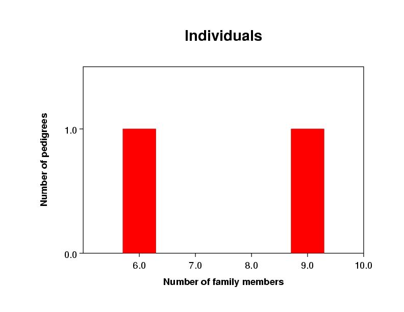
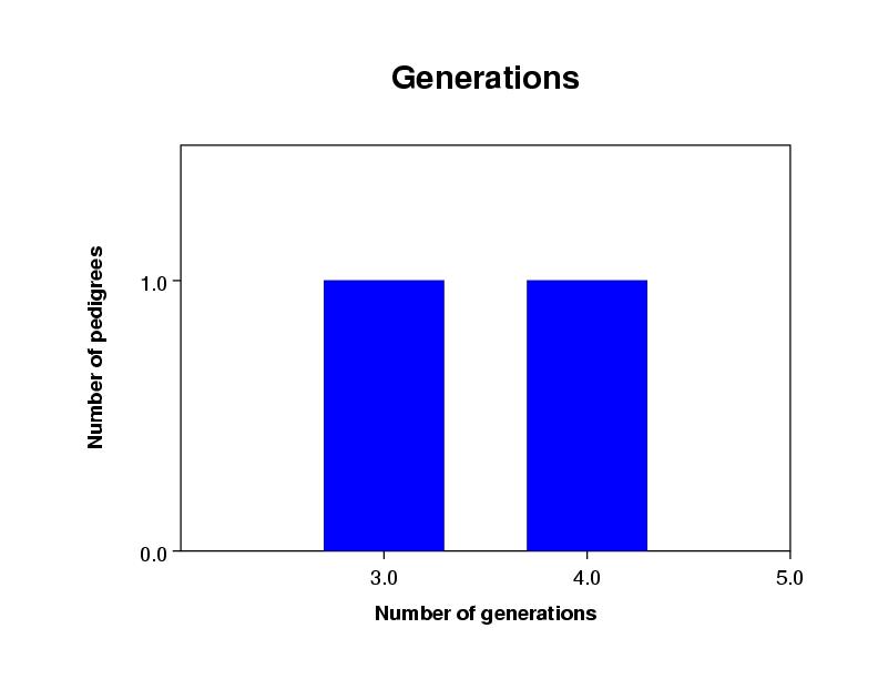
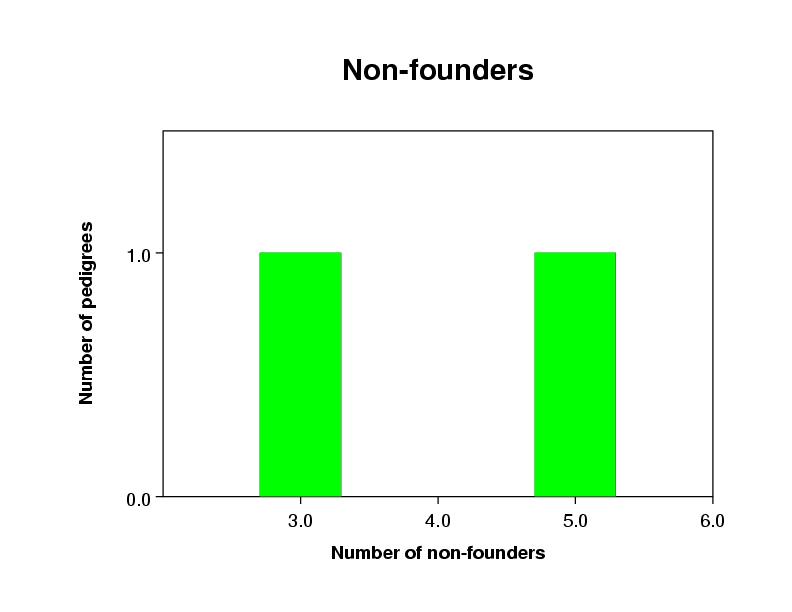
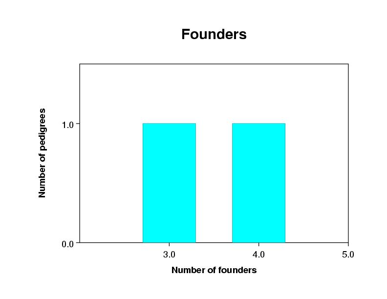
The first page of your PDF file will be a synopsis of the family structure of your pedigree file. A
typical result is shown below. The four histograms summarize the distributions of individuals
per family (upper left), generations per family
(upper right), non-founders per family (lower left) and
founders per family (lower right). By looking at these charts, you should be able to
verify that our sample includes 2 families with a total of 15 individuals, that one family has 3
generations and a second family has 4 generations, and that of the 15 individuals in our data set, 7 are founders
and 8 are non-founders.
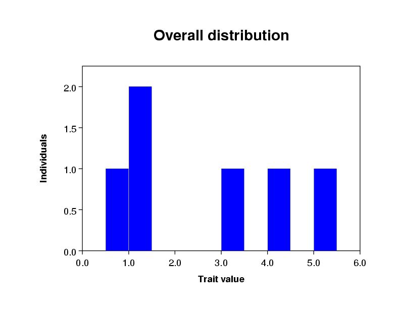
Distribution of covariate and quantitative trait values:
PEDSTATS creates one page of output for each covariate and quantitative trait specified in your pedigree file.
Using the output page below, you should be able to confirm that the sample mean
and variance of the quantititive trait some_trait are 2.63 and 3.64,
respectively. The overall distribution shows that the range of values for some_trait over
all phenotyped individuals in the sample is roughly 0.5 to 5.5, with one value in the range (0.5, 1.0), two in (1.0, 1.5), one in
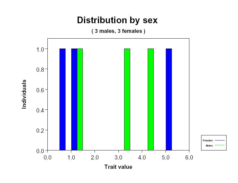
(3.0 ,3.5), one in (4, 4.5) and one in (5.0, 5.5). The distribution by sex shows that of the two
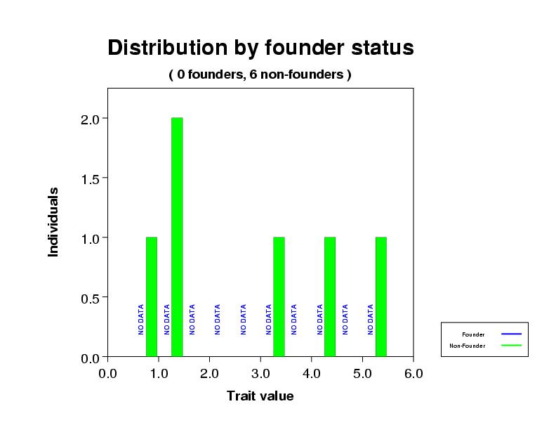
individuals with a value for some_trait falling in the range (1.0, 1.5), one is female and one is male. The distribution by founder status also shows that all six phenotyped individuals in the pedigree file
are non-founders and that none of the founders have been phenotyped for this trait.
The sib-sib plot in the lower left plots the trait value for each individual against the value
for each
cosib (sib in the same family). For purposes of this plot, sib pairs are ordered. For the current data, 8 data points
are plotted for the 4 phenotyped sib pairs; 2 for the 2 siblings in family 1 {(1.234, 4.321), (4.321, 1.234)}, and a total of six points for the 3
siblings in family 2 {( 1.234, 3.321) (1.234, 5.175), (3.321, 1.234), (3.321, 5.175), (5.175, 1.234), (5.175, 3.321)}
You'll also find the correlation between values for sib pairs in the title of sib-sib plot. This is calculated
using the formula
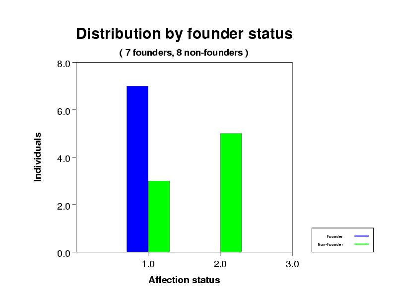
Affection status statistics
If affection status information is included in the pedigree file, PEDSTATS will generate a summary page for each characteristic. As
before, charts summarize sex-specific and founder-status
specific distributions of affection status as well as the distribution in the overall population.
The overall distribution indicates that among the 15 phenotyped individuals
in our sample, 10 individuals are unaffected. By looking at the distribution by founder
status, you can see that disease prevalence among founders in our sample is 0%. Among non-founders, prevalance is about 67.25%.
The histogram in the lower left (Sib Pairs) shows the distribution of
sib pairs across three affection categories
           Concordant, both unaffected               ( green )
           Discordant                                ( yellow )
           Concordant, both affected                 ( red )
In our dataset, family 1 has two affected sibs and therefore contributes one concordant, affected sib pair to the
total. Family 2 has three sibs (two affected, one unaffected) and
contributes 1 concordant, affected pair and 2 discordant pairs to the overall total of 2 concordant affected, 2 discordant,
and 0 concordant unaffected sib pairs.
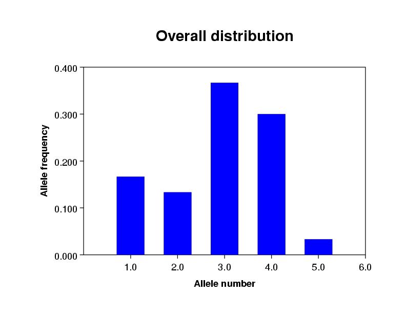
Marker allele frequencies
One page is generated for each marker locus in the pedigree file. If you check the overall distribution, you can see that 5 alleles (1, 2, 3,
4, 5) are present in our sample for the locus some_marker. Allele 3 is the most
common, with a frequency of 0.37 in the entire sample, while allele 5 is the least common with
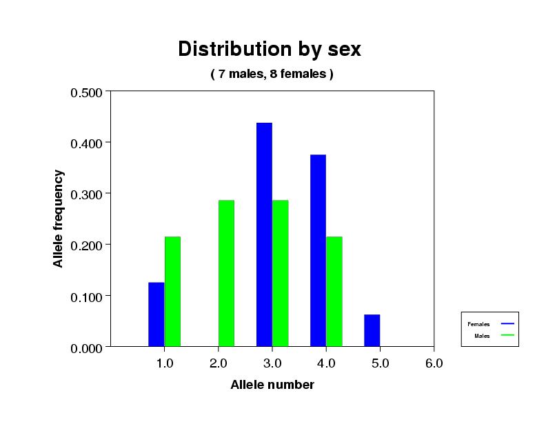
a frequency of about 0.03. The distribution by sex shows
that the frequencies differ somewhat between the sexes. If you believe in extrapolation from
tiny samples, you might note that in the male subsample, the frequencies of alleles 2 and 3
are roughly the same, whereas in the female sample, allele 3 is the most common followed by
allele 4. You might even notice that allele 5 isn't carried by any males.
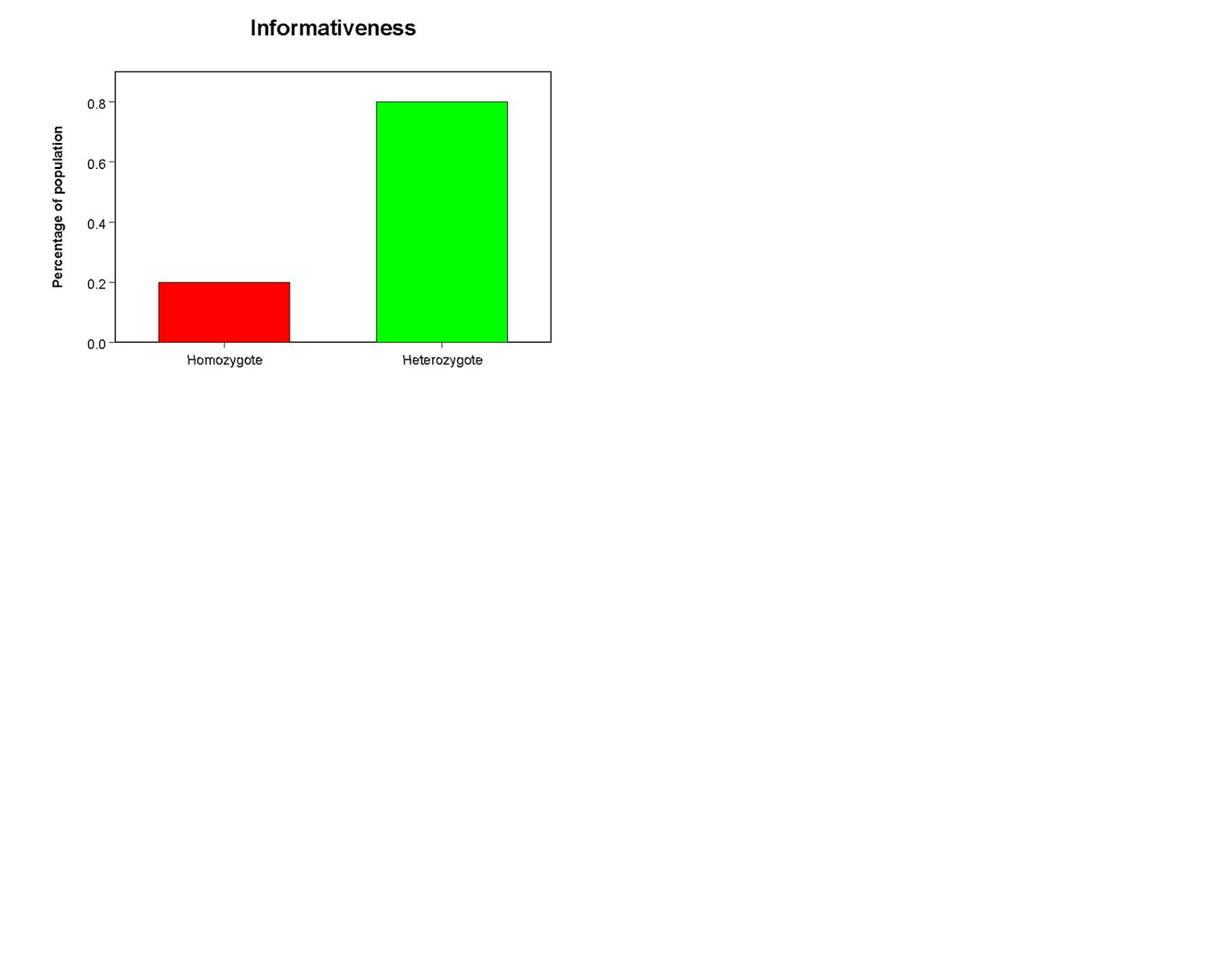
The Informativeness chart shows the percentage of genotyped at the current locus
individuals that are homozygous (in red) and heterozygous (in green). For the some_marker locus, 79% of the sample
is heterozygous and 21% is homozygous.
Now that you've seen some of the basic types of graphical output that PEDSTATS can create, you might
like to see some more interesting examples or take a look at some other types of
graphical output available (pairwise, sex-specific or
Hardy-Weinberg test results).
| |
